Numerical Relativity: Black Holes and Gravity - Part 3

 By: Unknown    6:47 PM  Christoffel symbols, deviation equation, Eddington-Finkelstein coordinates, general relativity, gravitational physics, metric, Minkowsky metric, Schwarzschild coordinates, spacetime, special relativity, tensors   No comments

Spacetime

The definition of spacetime comes from special relativity. It tells us that different inertial frames have different notions of time. Let's take three Cartesian coordinates (x, y, z). By moving these axes parallel to themselves from some origin, we create new values of x, y, and z. In addition, by moving these coordinates we are creating a notion of time, which is different in each of these inertial frames. This means that inertial frames are spanned by four coordinates (t, x, y, z).

Moving reference frames. Graphic from www.cv.nrao.edu.

Flat Spacetime and the Metric

Just like in geometry where we use the Pythagorean theorem, $  a^{2} + b^{2} =  c^{2} $ relativity uses something somewhat similar called a line element of flat spacetime $$  (\Delta s)^{2} = -(c\Delta t)^{2} + (\Delta x)^{2} + (\Delta y)^{2} + (\Delta z)^{2} $$ A line element, such as the one above, tells us the change in position vectors as time also changes. Combining these changes gives us the distance between points in spacetime - denoted by $ \Delta s $ . In fact, this is the one used in special relativity because it gives us flat spacetime (which is not true in general relativity). Since we have four coordinates that give us a quantity and a direction, they can be written as vectors and the  vectors can be written using index notation as shown below $$ \textbf{a} \cdotp \textbf{b} = (a^{\alpha} \textbf{e}_{\alpha}) \cdotp (b^{\beta} \textbf{e}_{\beta}) = (\textbf{e}_{\alpha} \cdotp \textbf{e}_{\beta}) a^{\alpha} b^{\beta} = \eta_{\alpha \beta} a^{\alpha} b^{\beta} $$ where $ \eta_{\alpha \beta} $ is the metric of flat space time and can be shown as a diagonal matrix

\(\eta_{\alpha \beta} =\begin{pmatrix}-c^2 & 0 & 0 & 0 \\ 0 & 1 & 0 & 0 \\ 0 & 0 & 1 & 0 \\ 0 & 0 & 0 & 1\end{pmatrix} =\begin{pmatrix}-1 & 0 & 0 & 0 \\ 0 & 1 & 0 & 0 \\ 0 & 0 & 1 & 0 \\ 0 & 0 & 0 & 1\end{pmatrix} = diag(-1,1,1,1)\)
Here the speed of light is made equal to one in order to make further calculations easier. This metric, called a Minkowsky metric, gives us information of the geometry and structure of spacetime. Although the matrix notation looks messy, it can be very useful for understanding calculations. Instead of writing $  (\Delta s)^{2} = \cdots $ we can just say $$  ds^{2} = \eta_{\alpha\beta} dx^{\alpha} dx^{\beta} $$ The reason why we changed $ \Delta $ into $ d $ is to show that the values are now changing by infinitesimal amounts. Our $ \alpha 's $ and $ \beta 's $ sum over our four coordinates. I recommend learning about Einstein notation so that the formula above becomes clearer. This notation will prove crucial in the posts of gr-qc publications.

Curved Spacetime and the Coordinate Problem

**NOTE: The gravitational constant, G, and the speed of light, c, will be equal to one from now on.** 

Inertial frames are useful because of the special symmetries of flat spacetime. However, in general relativity spacetime is curved and, generally, not symmetric. This means that we cannot take one coordinate system (and I am not talking only about Cartesian or spherical) to simplify the laws; instead, we have to chose a specific system for a specific problem. For example, if we use Schwarzschild coordinates (below)
$$ ds^2 = - \left( 1 - \frac{2M}{r} \right)dt^2 + \left(1 - \frac{2M}{r} \right)^{-1}dr^2 + r^2(d \theta ^2 + sin^2{\theta} d \phi^2) $$
we will find that it breaks down at r = 2M, 0. If instead we decide to use Eddington-Finkelstein coordinates (below)
$$ ds^2 = - \left( 1 - \frac{2M}{r} \right)dv^2 + 2dvdr + r^2(d \theta ^2 + sin^2{\theta} d \phi^2) $$ we will only get infinity at the physical singularity - when at r = 0. This shows us that sometimes, we just need to use a different coordinate system, and there is not one that can be used to solve all problems.

Just as we use Maxwell's equations for electromagnetic fields, we use Einstein's equation for gravitational fields. Einstein's equation is a set of ten second-order partial differential equations; they are also nonlinear. This set of equations tell us how a measure of local spacetime curvature is related to a measure of matter energy density. To find a measure of spacetime curvature, we must come up with a thought experiment on the motion of at least two test particles. Imagine two rings of test particles, one is in space and the other is falling towards the Earth. The particles in space feel no force, so they stay in the shape of a ring. However, the ones experiencing the Earth's gravitational force will start forming an ellipse. This occurs because the particles closer to the Earth feel a stronger pull than the ones further away, and the particles on the sides of the falling ring will begin to come closer together since they are pulled towards the center of the Earth. This change of shape in the rings is a measure of spacetime curvature. This is exactly what Newtonian gravity dictates and the derivation is short.

Unlike the Newtonian view, Einstein saw that the relative accelerations of these particles are not caused by changes in the gravitational force, but instead, they are caused by the fact that particles simply follow geodesics, or straight lines, in spacetime. And because we are seeing these particles accelerate, their geodesics must be curving relative to each other. This shows us that spacetime is actually being curved. To follow the derivation of the equation of geodesic deviation in general relativity and understand the implications in-depth, you must understand the use and meaning of Einstein notation, tensors, and Christoffel symbols. You will be able to follow the math without knowing about Christoffel symbols. In the derivations linked below, I will explain as much as I can without going off topic. While the first link is easier to follow, the second link will be mathematically rigorous.

Links from above:

1. Derivation of the Newtonian Deviation Equation

2. Derivation of the Geodesic Deviation Equation 

Derivation of the Equation of Geodesic Deviation

 By: Unknown    6:47 PM  Christoffel symbols, deviation equation, Einstein, general relativity, geodesic, gravitational physics, gravity, Riemann curvature, tensors   No comments

Because this derivation is often given as homework in classes that teach relativity, I will not show step-by-step derivations. Instead, I will only show the steps that books tend to give. If you are confident in your use of tensor notation, you shouldn't have a problem filling in the steps. However, it can get extremely messy when it calls for a change in indices. I will again reference "A General Relativity Workbook" by Thomas A. Moore.

[Here is a "punny" article on tensors.]

We use tensors in this derivation so that it is valid in arbitrary coordinates. Let's go back to our particles and define their positions by $ x^{\alpha}(\tau) $ and $ \bar{x}^{\alpha}(\tau) \equiv x^{\alpha}(\tau) + n^{\alpha}(\tau) $, where $ \tau $ is our proper time and $ \textbf{n} $ is our infinitesimal separation four-vector. Keep in mind that although this derivation is similar to that in Newtonian mechanics, this derivation uses relativistic concepts. Just as with the Newtonian derivation, we must write expressions that govern the motion of both particles along their geodesics.

$$ 0 = \frac{d^2 x^{\alpha}}{d \tau^2} + \Gamma^{\alpha}_{\mu \nu} \frac{dx^{\mu}}{d \tau} \frac{dx^{\nu}}{d \tau} , \qquad 0 = \frac{d^2 \bar{x}^{\alpha}}{d \tau^2} + \bar{\Gamma}^{\alpha}_{\mu \nu} \frac{d \bar{x}^{\mu}}{d \tau} \frac{d \bar{x}^{\nu}}{d \tau} $$

Here, we express the particles' coordinate accelerations in terms of the Christoffel symbols instead of having them in terms of the gravitational potential. Christoffel symbols are combinations of first derivatives of the metric that describe effects of parallel transport in manifolds. Just like we did in the Newtonian derivation, we can use Taylor series to expand Christoffel symbol of the second particle around the value of the first particle since the separations are infinitesimal (shown below). 

$$ \bar{\Gamma}^{\alpha}_{\mu \nu} (at \: \bar{x}^{\alpha} (\tau)) \approx \Gamma^{\alpha}_{\mu \nu} (at \: x^{\alpha} (\tau)) + n^{\sigma} [ \partial_{\sigma} \Gamma^{\alpha}_{\mu \nu}] (at \: x^{\alpha} (\tau)) $$

Now, we know $ \bar{x}^{\alpha}(\tau) \equiv x^{\alpha}(\tau) + n^{\alpha}(\tau) $ so we will plug this and the expansion above into the equation of motion of the second particle which gives us

$$ 0 = \frac{d^2 (x^{\alpha} + n^{\alpha})}{d \tau^2} + [\Gamma^{\alpha}_{\mu \nu} + n^{\sigma} ( \partial_{\sigma} \Gamma^{\alpha}_{\mu \nu})] \frac{d (x^{\mu} + n^{\mu})}{d \tau} \frac{d (x^{\nu} + n^{\nu})}{d \tau} $$

$$  \qquad \qquad \; \; = \frac{d^2 x^{\alpha}}{d \tau^2} + \frac{d^2 n^{\alpha}}{d \tau^2} + [\Gamma^{\alpha}_{\mu \nu} + n^{\sigma} ( \partial_{\sigma} \Gamma^{\alpha}_{\mu \nu})] \left( \frac{d x^{\mu}}{d \tau} + \frac{d n^{\mu}}{d \tau} \right) \left( \frac{d x^{\nu}}{d \tau} + \frac{d n^{\nu}}{d \tau} \right) $$

We want to simplify this more by multiplying out everything and using our geodesic equations. Doing this will give us

$$ ** \quad 0 = \frac{d^2 n^{\alpha}}{d \tau^2} + 2 \Gamma^{\alpha}_{\mu \nu} u^{\mu} \frac{d n^{\nu}}{d \tau} + n^{\sigma} ( \partial_{\sigma} \Gamma^{\alpha}_{\mu \nu} u^{\mu}) u^{\mu} u^{\nu} $$

where $ u^{\mu} \equiv \frac{d x^{\mu}}{d \tau} $ is the first particle's four-velocity. Because this is  a four-vector we know that its derivative with respect to $ \tau $ is

$$ \left( \frac{d \textbf{n}}{d \tau} \right)^{\alpha} = \frac{d n^{\alpha}}{d \tau} + \Gamma^{\alpha}_{\mu \nu} u^{\mu} n^{\nu} $$

and so we take the second derivative and find it to be

$$ \left( \frac{d^2 \textbf{n}}{d \tau^2} \right)^{\alpha} = \left( \frac{d}{d \tau} \left[ \frac{d \textbf{n}}{d \tau} \right] \right)^{\alpha} = \frac{d}{d \tau} \left( \frac{d n^{\alpha}}{d \tau} + \Gamma^{\alpha}_{\mu \nu} u^{\mu} n^{\nu} \right) + \Gamma^{\alpha}_{\sigma \nu} u^{\sigma} \left( \frac{d n^{\nu}}{d \tau} + \Gamma^{\nu}_{\beta \gamma} u^{\beta} n^{\gamma} \right) $$

$$ = \frac{d^2 n^{\alpha}}{d \tau^2} + \frac{d \Gamma^{\alpha}_{\mu \nu}}{d \tau} u^{\mu} n^{\nu} + \Gamma^{\alpha}_{\mu \nu} \frac{d u^{\mu}}{d \tau} n^{\nu} + \Gamma^{\alpha}_{\mu \nu} u^{\mu} \frac{d n^{\nu}}{d \tau} + \Gamma^{\alpha}_{\sigma \nu} u^{\sigma} \frac{d n^{\nu}}{d \tau} + \Gamma^{\alpha}_{\sigma \nu} \Gamma^{\nu}_{\beta \gamma} u^{\sigma} u^{\beta} n^{\gamma} $$

Now, this is getting really messy so let us simplify by noticing two key things:

$$ 1. \frac{d \Gamma^{\alpha}_{\mu \nu}}{d \tau} = \frac{d x^{\sigma}}{d \tau} \frac{\partial \Gamma^{\alpha}_{\mu \nu}}{\partial x^{\sigma}} = u^{\sigma} \partial_{\sigma} \Gamma^{\alpha}_{\mu \nu} $$

$$ 2. \; Changing \; \sigma \; to  \; \mu \; will \; make \; two \; of \; the \; terms \; the \; same. $$

Using both of these in the messy equation we have so far simplifies it to

$$ \left( \frac{d^2 \textbf{n}}{d \tau^2} \right)^{\alpha} = \frac{d^2 n^{\alpha}}{d \tau^2} + \left( \partial_{\sigma} \Gamma^{\alpha}_{\mu \nu} \right) u^{\sigma} u^{\mu} n^{\nu} + \Gamma^{\alpha}_{\mu \nu} \frac{d u^{\mu}}{d \tau} n^{\nu} + 2 \Gamma^{\alpha}_{\mu \nu} u^{\mu} \frac{d n^{\nu}}{d \tau} + \Gamma^{\alpha}_{\sigma \nu} \Gamma^{\nu}_{\beta \gamma} u^{\sigma} u^{\beta} n^{\gamma} $$

Ok, so now the tricky part comes. We need to do three things: use the geodesic equation of the first particle to eliminate $ \frac{d u^{\mu}}{d \tau} $, use the equation labeled with ** in order to eliminate $ \frac{d^2 n^{\alpha}}{d \tau^2} $, and rename indices to pull out a common factor of $ u^{\sigma} u^{\mu} n^{\nu} $. This will take a while. The trickiest part is definitely changing the indices because there are so many of them. Try to see what you can cancel out and remember the symmetries of the Christoffel symbols. After this, we will get

$$ \left( \frac{d^2 \textbf{n}}{d \tau^2} \right)^{\alpha} = \left( \partial_{\sigma} \Gamma^{\alpha}_{\mu \nu} - \partial_{\nu} \Gamma^{\alpha}_{\mu \sigma} + \Gamma^{\alpha}_{\sigma \gamma} \Gamma^{\gamma}_{\mu \nu} - \Gamma^{\alpha}_{\nu \gamma} \Gamma^{\gamma}_{\mu \sigma} \right) u^{\sigma} u^{\mu} n^{\nu} $$

Since the left side is a tensor and everything outside the parenthesis on the right side is a tensor, then the stuff inside the parenthesis must be a tensor. Not surprisingly, the stuff inside is actually the Riemann tensor, but with the signs flipped. So the Riemann tensor, which is the measure of spacetime curvature, is defined as

$$ R^{\alpha}_{\mu \nu \sigma} \equiv \partial_{\nu} \Gamma^{\alpha}_{\mu \sigma} - \partial_{\sigma} \Gamma^{\alpha}_{\mu \nu} + \Gamma^{\alpha}_{\nu \gamma} \Gamma^{\gamma}_{\mu \sigma} - \Gamma^{\alpha}_{\sigma \gamma} \Gamma^{\gamma}_{\mu \nu} $$

Therefore, we can rewrite the last equation using the Riemann definition and we get

$$ \left( \frac{d^2 \textbf{n}}{d \tau^2} \right)^{\alpha} = - R^{\alpha}_{\mu \nu \sigma} u^{\sigma} u^{\mu} n^{\nu} $$

This is the Geodesic Deviation Equation. This is extremely useful because it allows us to see if spacetime is flat or curved, which we can't do by looking at the metric. So if the any of the components of the Riemann tensor are non-zero, then spacetime is curved.

Numerical Relativity: Black Holes and Gravity - Part 2

 By: Unknown    9:55 PM  astrophysics, black holes, Einstein, general relativity, gravitational collapse, gravitational physics, gravitational waves, radiation, spacetime   No comments

Einstein's Theory of General Relativity

You have probably heard about Einstein's Theory of Relativity. His work on special relativity was published in 1905. This introduced a new framework in physics. He showed that the laws of physics are the same in all non-accelerating reference frame and that the speed of light is constant. This revolutionized different branches of physics and led to his 1915 Theory of General Relativity, or his theory of gravity. Einstein's view was that space and time could be distorted by objects with mass. This spacetime would be able to be stretched and bent. A classic example of this is to imagine a heavy object in the middle of a trampoline. Spacetime is distorted just like the fabric of the trampoline. This would change the way we perceive space and time. Perhaps the most outstanding predictions of this theory are black holes and gravitational waves.

Black Holes (BHs)

In the media, black holes are erroneously described as giant vacuum cleaners in space. Black holes do not suck in things in the way vacuum cleaners do. Physicist instead think of black holes as regions in space with extreme curvature. Black holes warp space and time in such an extreme manner that nothing - not even light - can escape once it is caught into orbit. Since light can't escape it, we cannot look up at the sky and actually point at a black hole. Instead we use different methods to find them. For example, we look for an object orbiting some dark region of space. We will discuss this further in a future post.

Black Hole Anatomy

Let's look at the anatomy of a black hole. Although a black hole is not an actual object we can touch, let's think of it as a black sphere; we choose black since we can't see black holes in the sky. First, let's call the surface of the sphere the event horizon. Once anything passes this point, it cannot return outside. In fact, we don't even know what happens inside the event horizon. All that we know is that there is a point inside which we call a singularity. A singularity is when the gravitational field is at infinity. This is where physics breaks down.

How Do Black Holes Form?

There are three main ways in which black holes form: implosion, high-energy collision, and binary black hole (BBH) collisions. Implosion, or gravitational collapse, is perhaps the most talked about way of black hole formation. This occurs when a star that is a few times larger than the size of our sun collapse onto itself due to a greater gravitation (or inward) force and smaller internal pressure (outward force). I will mention that for a star to implode, there is a minimum size, which is about 3 solar masses. This Tolman-Oppenheimer-Volkoff limit, however, is not well known because it depends on the equations of state for matter this dense, i.e. the relationship between the volume, pressure, temperature, and internal energy of a star.

Diagram of gravitational force vs. internal pressure on a star .

I won't go into details on the formation by high-energy collisions, since this could only happen in very special conditions. This type of event has never been detected, so it is purely theoretical. If it actually ever happened, the black hole would be so small that it would evaporate extremely fast.

Formation by binary black hole collisions is in a way the "easiest" to understand. Unlike implosion where there is an actual birth of a black hole, this type of collisions involve two already formed black holes that collide in order to form a bigger black hole. A very cool thing about this is that the final mass of this black hole is not equal to that of the sum of the two initial black holes. You might be wondering why! The next section gives us the answer.

Gravitational Waves (GWs)

Fantastic! So in the paragraph above we asked why the mass of the final black hole is not the sum of the two initial black holes that collided. This is actually my research area now, so I will try to explain it very thoroughly.

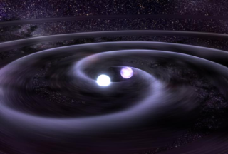
Gravitational waves, or gravitational radiation, are a result of acceleration; it is like light only in the sense that both types of radiation carry energy away. A great example of this is a system of two black holes. When two massive bodies orbit around each other, they accelerate. Because our system must conserve energy, gravitational radiation must be given off as our BHs accelerate, and this draws our BHs closer together which causes them to orbit faster. This radiation distorts spacetime, which is why you might have heard of the definition "Gravitational waves are ripples in spacetime." The closer they are, the more strongly radiate.

Binary neutron stars orbiting each other and radiating. Photo taken from NASA.

Below, you can see a picture of this radiation as the black holes get closer to each other and eventually collide. The height is the amplitude of the gravitational waves. the length shows the passing of time. Evidently, gravitational waves are given off as the BHs orbit each other. As they get closer the radiation increases by large factor. The highest point you see in the wave above, shows the time at which the black holes collided to become one. This releases an incredible amount of energy, making a BBH collision the most energetic phenomena in space. After they collide, the final BH will ring like a bell (radiating more) and eventually dying down to a quiescent state. When a black hole is not moving or "eating" anything, it will not radiate. 

Gravitational wave from a BBH.

I will go into more detail on how to detect this waves and what we can learn about them in a future post.